November 2020 – N N Taleb's Probability Notebook

Every study needs its own statistical tools, adapted to the specific problem, which is why it is a good practice to require that statisticians come from mathematical probability rather than some software-cookbook school. When one uses canned software statistics adapted to regular medicine (say, cardiology), one is bound to make severe mistakes when it comes to epidemiological problems in the tails or ones where there is a measurement error. The authors of the study discussed below (The Danish Mask Study) both missed the effect of false positive noise on sample size and a central statistical signal from a divergence in PCR results. A correct computation of the odds ratio shows a massive risk reduction coming from masks.

The article by Bundgaard et al., [“Effectiveness of Adding a Mask Recommendation to Other Public Health Measures to Prevent SARS-CoV-2 Infection in Danish Mask Wearers”, Annals of Internal Medicine (henceforth the “Danish Mask Study”)] relies on the standard methods of randomized control trials to establish the difference between the rate of infections of people wearing masks outside the house v.s. those who don’t (the control group), everything else maintained constant.
The authors claimed that they calibrated their sample size to compute a p-value (alas) off a base rate of 2% infection in the general population.
The result is a small difference in the rate of infection in favor of masks (2.1% vs 1.8%, or 42/2392 vs. 53/2470), deemed by the authors as not sufficient to warrant a conclusion about the effectiveness of masks.

We would like to alert the scientific community to the following :

The Mask Group has 0/2392 PCR infections vs 5/2470 for the Control Group. Note that this is the only robust result and the authors did not test to see how nonrandom that can be. They missed on the strongest statistical signal. (One may also see 5 infections vs. 15 if, in addition, one accounts for clinically detected infections.)

The rest, 42/2392 vs. 53/2470, are from antibody tests with a high error rate which need to be incorporated via propagation of uncertainty-style methods on the statistical significance of the results. Intuitively a false positive rate with an expected “true value” $p$ is a random variable $\rightarrow$ Binomial Distribution with STD $\sqrt{n p (1-p)}$ , etc.
False positives must be deducted in the computation of the odds ratio.
The central problem is that both p and the incidence of infection are in the tails!

Immediate result: the study is highly underpowered –except ironically for the PCR and PCR+clinical results that are overwhelming in evidence.

Further:

As most infections happen at home, the study does not inform on masks in general –it uses wrong denominators for the computation of odds ratios (mixes conditional and unconditional risk). Worse, the study is not even applicable to derive information on masks vs. no masks outside the house since during most of the study (April 3 to May 20, 2020), “cafés and restaurants were closed “, conditions too specific and during which the infection rates are severely reduced –tells us nothing about changes in indoor activity. (The study ended June 2, 2020). A study is supposed to isolate a source of risk; such source must be general to periods outside the study (unlike cardiology with unconditional effects).
The study does not take into account the fact that masks might protect others. Clearly this is not cardiology but an interactive system.
Statistical signals compound. One needs to input the entire shebang, not simple individual tests to assess the joint probability of an effect.

Now, some quick technical derivations.

Distribution of the sample under type 2 error

Simple method: Let $X, Y, Z$ be random variables in $\{0,1\}$ ; we have

$\underbrace{x_1, x_2, \ldots, x_{m_1}}_{\text{real positive}}+\underbrace{y_1, y_2, \ldots, y_{m_2}}_{\text{false positive}}+ \underbrace{z_1, z_2, \ldots, z_{m_3}}_{\text{false and true negative}}$

with the constraint that $m_1+m_2 \leq n$ .

So $\{m_1, m_2, m_3\}$ follow a multinomial distribution with probabilities $\{p_1,p_2, p_3\}$ .

If we consider $m_1 + m_2$ , the observable incidence in each group, the variable follows a binomial distribution $B(n, \frac{m_1+m_2}{n})$ , with a large share of the variance coming from $m_2$ .

This poses an immediate problem: we are concerned with $m_1$ not $m_1+m_2$ . The odds ratio in each sample used by the researchrs is $\frac{m_1^M+m_2^M}{m_1^N+m_2^N}$ (where M is for the mask condition and N the no mask one); it is diluted by $m_2$ , which can be considerable.

A back of the envelope analysis shows that, in the presence of a false positive rate of just 1%, we have a large gain for masks. It would not be 42/2392 vs. 53/2470 but rather, by adding the known true positives and reducing by the false negatives (approximately):

$\frac{42-24+5- \text{home infections}}{2392}$ vs $\frac{53- 24.7+15-\text{home infections}}{2470}$ ,

which is at least an overall drop in 47% of incidence for masks, not counting home infections, which, if they were just 1% (half the total claimed by the resarchers), would increase the benefits for masks in a yuuuuuuuge way (up to 100%).

(These numbers are preliminary and need refining).

More advanced method: Let the initial incidence rate $X \sim \mathcal{N} (\mu , s)$ (a Gaussian) for a given sample n. Let us incorporate the false negative as all values across. Let $n$ be the total sample size, $p$ the (net) probability of a false positive. We now have $f(.)$ the corrected distribution of the revealed infection count (using a Binomial distribution of the net false positive rate).

$f (x)=\sum _{m=1}^n \frac{p^m \binom{n}{m} (1-p)^{n-m} e^{-\frac{(-m-p+x)^2}{2 s^2}}}{\sqrt{2 \pi } s}$

Under normal approximation to the binomial:

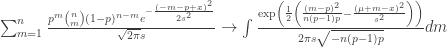
$\sum _{m=1}^n \frac{p^m \binom{n}{m} (1-p)^{n-m} e^{-\frac{(-m-p+x)^2}{2 s^2}}}{\sqrt{2 \pi } s} \rightarrow \int \frac{\exp \left(\frac{1}{2} \left(\frac{(m-p)^2}{n (p-1) p}-\frac{(\mu +m-x)^2}{s^2}\right)\right)}{2 \pi s \sqrt{-n (p-1) p}} dm$

Allora

$f (x)=\frac{e^{\frac{(\mu +p-x)^2}{2 n (p-1) p-2 s^2}}}{s \sqrt{2 \pi -\frac{2 \pi n (p-1) p}{s^2}}},$

which appears to be Gaussian. For we have:

$\mathbb{E} (X)=\mu +p$

$\mathbb{V}(X)=s^2+n p (1-p)$

$\mathbb{E}(X^4)=3 (-n (-1 + p) p + s^2)^2$ , hence the kurtosis is that of a Gaussian.

As you see the variance goes through the roof. More details would show that the study needs at least 4 times the sample size for the same approach. I have not added false negatives, but these too would increase the variance.

Considerations on the 0/5 PCR results

Now consider the more obvious error. What are the odds of getting 0 PCRs vs 5 from random?

The probability of having 0 realizations in 2392 if the mean is $\frac{5}{2470}$ is 0.0078518, that is 1 in 127. We can reexpress it in p values, which would be well <.05, that is far in excess of the ps in the range .21-.33 that the paper shows. How these researchers missed the point is beyond me.

PMF of a binomial distribution(2392 , $\frac{5}{2470}$ ) .

Pegadogical presentation of a draw of 5 with the {0,5} combination

Monte Carlo Analysis, again another way.

More textbook-style Fisher approach, similar to our heuristic

Considerations on the 5/15 PCR+Clinial detection results

Now consider the 5 vs. 15 PCR + (adjusting the rest)

PMF of a binomial distribution(2392 , $\frac{15}{2470}$ ) .

Clinically detected Covid.

The probability of having 5 or less realizations in 2392 if the mean is $\frac{15}{2470}$ is 0.00379352, that is 1 in 263. We can reexpress it in p values, which would be well <.1 [CORRECTED based on comments].

(To be continued. I wonder why the journal published a paper with already weak p values, without asking for a repeat with a larger sample which can cure the deficit.)