Maximum Ignorance Probability, with application to surgery’s error rates

Introduction and Result

A maximum entropy alternative to Bayesian methods for the estimation of independent Bernouilli sums.

Let , where be a vector representing an n sample of independent Bernouilli distributed random variables . We are interested in the estimation of the probability p.

We propose that the probablity that provides the best statistical overview, (by reflecting the maximum ignorance point) is

, (1)

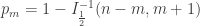
where and is the beta regularized function.

Comparison to Alternative Methods

EMPIRICAL: The sample frequency corresponding to the “empirical” distribution , which clearly does not provide information for small samples.

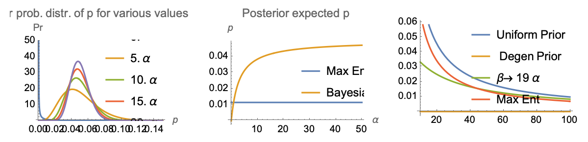
BAYESIAN: The standard Bayesian approach is to start with, for prior, the parametrized Beta Distribution , which is not trivial: one is contrained by the fact that matching the mean and variance of the Beta distribution constrains the shape of the prior. Then it becomes convenient that the Beta, being a conjugate prior, updates into the same distribution with new parameters. Allora, with n samples and m realizations:

(2)

with mean . We will see below how a low variance beta has too much impact on the result.

Derivations

Let be the CDF of the binomial . We are interested in the maximum entropy probability. First let us figure out the target value q.

To get the maximum entropy probability, we need to maximize . This is a very standard result: taking the first derivative w.r. to q, and since is concave to q, we get .

Now we must find p by inverting the CDF. Allora for the general case,

.

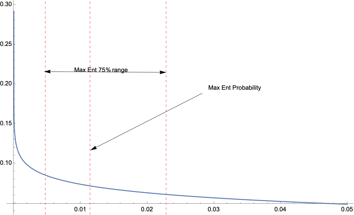
And note that as in the graph below (thanks to comments below by überstatistician Andrew Gelman), we can have a “confidence band” (sort of) with

;

in the graph below the band is for values of: .

Application: What can we say about a specific doctor or center’s error rate based on n observations?

Case (Real World): A thoraxic surgeon who does mostly cardiac and lung transplants (in addition to emergency bypass and aortic ruptures) operates in a business with around 5% perioperative mortality. So far in his new position in the U.S. he has done 60 surgeries with 0 mortality.

What can we reasonable say, statistically, about his error probability?

Note that there may be selection bias in his unit, which is no problem for our analysis: the probability we get is conditional on being selected to be operated on by that specific doctor in that specific unit.

Assuming independence, we are concerned with a binomially distributed r.v. where n is the number of trials and is the probability of failure per trial. Clearly, we have no idea what p and need to produce our best estimate conditional on, here, .

Here applying (1) with and , we have .

Why is this preferable to a Bayesian approach when, say, n is moderately large?

A Bayesian would start with a prior expectation of, say .05, and update based on information. But it is highly arbitrary. Since the mean is , we can eliminate one parameter. Let us say we start with and have no idea of the variance. As we can see in the graph below there are a lot of shapes to the possible distribution: it becomes all in the parametrization.

APPENDIX: JAYNES’ BRANDEIS PROBLEM

When I worked on this problem, and posted the initial derivations, I wasn’t aware of Jaynes’ “Brandeis Problem”. It is not the same as mine as it ignores n and it led to a dead-end because the multinomial is unwieldy. But his approach would have easily let to more work if we had computational abilities then (maximization, as one can see below, can be seamless).

Acknowledgments

Thanks to Saar Wilf for useful discussions.