Figuring out the sampling error of rolling correlation.
Financial theory requires correlation to be constant (or, at least, known and nonrandom). Nonrandom means predictable with waning sampling error over the period concerned. Ellipticality is a condition more necessary than thin tails, recall my Twitter fight with that non-probabilist Clifford Asness where I questioned not just his empirical claims and his real-life record, but his own theoretical rigor and the use by that idiot Antti Ilmanen of cartoon models to prove a point about tail hedging. Their entire business reposes on that ghost model of correlation-diversification from modern portfolio theory. The fight was interesting sociologically, but not technically. What is interesting technically is the thingy below.
How do we extract sampling error of a rolling correlation? My coauthor and I could not find it in the literature so we derive the test statistics. The result: it has less than odds of being sampling error.
The derivations are as follows:
Let and be independent Gaussian variables centered to a mean . Let be the operator.
\
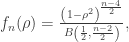
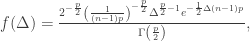
First, we consider the distribution of the Pearson correlation for observations of pairs assuming (the mean is of no relevance as we are focusing on the second moment):
with characteristic function:
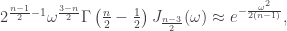
where is the Bessel J function.
We can assert that, for sufficiently large: the corresponding characteristic function of the Gaussian.
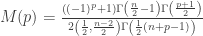
Moments of order become:
where is the Beta function. The standard deviation is and the kurtosis .
This allows us to treat the distribution of as Gaussian, and given infinite divisibility, derive the variation of the component, sagain of (hence simplify by using the second moment in place of the variance):.
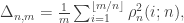
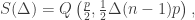
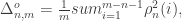
To test how the second moment of the sample coefficient compares to that of a random series, and thanks to the assumption of a mean of , define the squares for nonoverlapping correlations:
where is the sample size and is the correlation window. Now we can show that:
where and is the Gamma distribution with PDF: and survival function:
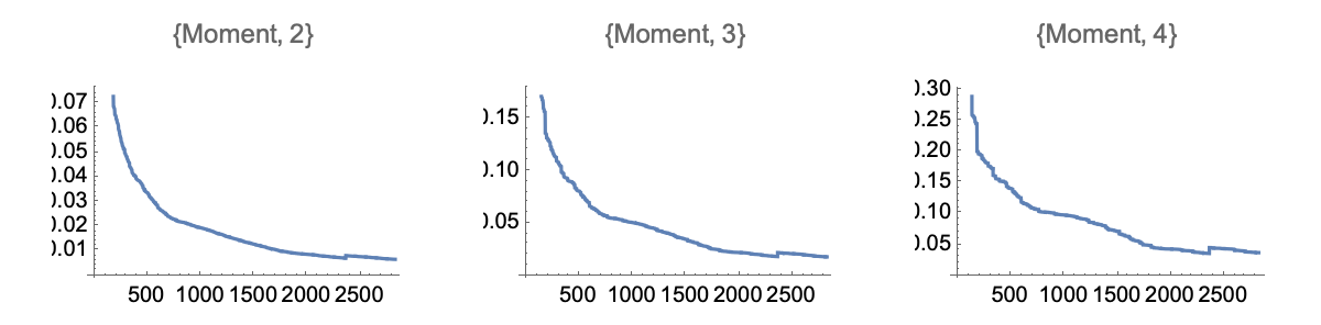
which allows us to obtain p-values below, using observations (and using the leading order $O(.)$:
Such low p-values exclude any controversy as to their effectiveness cite{taleb2016meta}.
We can also compare rolling correlations using a Monte Carlo for the null with practically the same results (given the exceedingly low p-values). We simulate with overlapping observations:
Rolling windows have the same second moment, but a mildly more compressed distribution since the observations of over overlapping windows of length are autocorrelated (with, we note, an autocorrelation between two observations orders apart of ). As shown in the figure below for we get exceedingly low p-values of order .
A maximum entropy alternative to Bayesian methods for the estimation of independent Bernouilli sums.
Let , where be a vector representing an n sample of independent Bernouilli distributed random variables . We are interested in the estimation of the probability p.
We propose that the probablity that provides the best statistical overview, (by reflecting the maximum ignorance point) is
, (1)
where and is the beta regularized function.
Comparison to Alternative Methods
EMPIRICAL: The sample frequency corresponding to the “empirical” distribution , which clearly does not provide information for small samples.
BAYESIAN: The standard Bayesian approach is to start with, for prior, the parametrized Beta Distribution , which is not trivial: one is contrained by the fact that matching the mean and variance of the Beta distribution constrains the shape of the prior. Then it becomes convenient that the Beta, being a conjugate prior, updates into the same distribution with new parameters. Allora, with n samples and m realizations:
(2)
with mean . We will see below how a low variance beta has too much impact on the result.
Derivations
Let be the CDF of the binomial . We are interested in the maximum entropy probability. First let us figure out the target value q.
To get the maximum entropy probability, we need to maximize . This is a very standard result: taking the first derivative w.r. to q, and since is concave to q, we get .
Now we must find p by inverting the CDF. Allora for the general case,
.
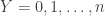
And note that as in the graph below (thanks to comments below by überstatistician Andrew Gelman), we can have a “confidence band” (sort of) with
;
in the graph below the band is for values of: .
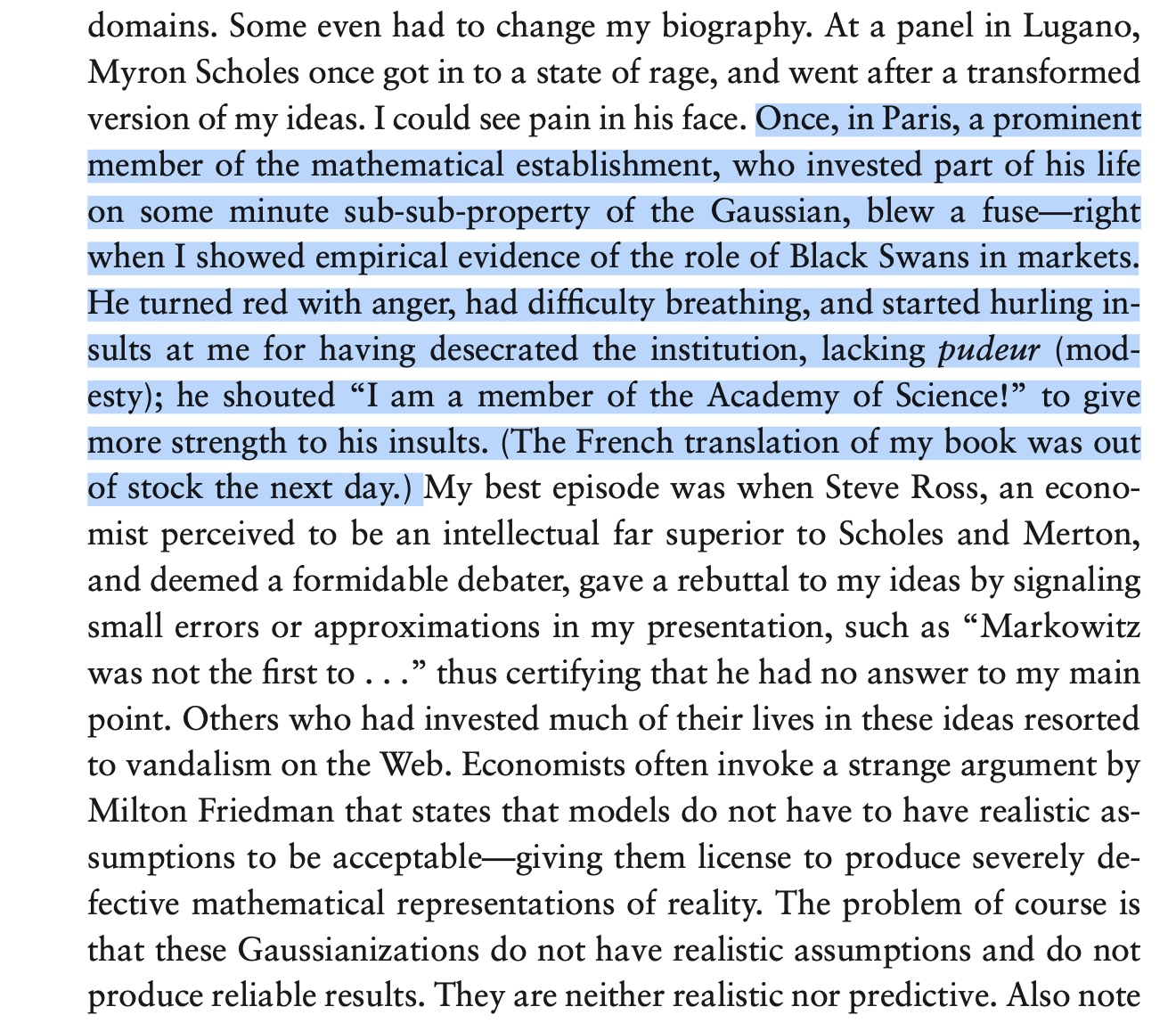
Application: What can we say about a specific doctor or center’s error rate based on n observations?
Case (Real World): A thoraxic surgeon who does mostly cardiac and lung transplants (in addition to emergency bypass and aortic ruptures) operates in a business with around 5% perioperative mortality. So far in his new position in the U.S. he has done 60 surgeries with 0 mortality.
What can we reasonable say, statistically, about his error probability?
Note that there may be selection bias in his unit, which is no problem for our analysis: the probability we get is conditional on being selected to be operated on by that specific doctor in that specific unit.
Assuming independence, we are concerned with a binomially distributed r.v. where n is the number of trials and is the probability of failure per trial. Clearly, we have no idea what p and need to produce our best estimate conditional on, here, .
Here applying (1) with and , we have .
Why is this preferable to a Bayesian approach when, say, n is moderately large?
A Bayesian would start with a prior expectation of, say .05, and update based on information. But it is highly arbitrary. Since the mean is , we can eliminate one parameter. Let us say we start with and have no idea of the variance. As we can see in the graph below there are a lot of shapes to the possible distribution: it becomes all in the parametrization.
APPENDIX: JAYNES’ BRANDEIS PROBLEM
When I worked on this problem, and posted the initial derivations, I wasn’t aware of Jaynes’ “Brandeis Problem”. It is not the same as mine as it ignores n and it led to a dead-end because the multinomial is unwieldy. But his approach would have easily let to more work if we had computational abilities then (maximization, as one can see below, can be seamless).
So far I received only one sound piece of criticism, by the financial economist Gur Huberman. Just as a painting has a utility to a collector, akin to a consumer good, bitcoin has utility for… fraudsters.
This is indeed correct but somehow it still doesn’t make much difference. Why? Because, it is turning out, bitcoin is way too transparent for a real fraudster to escape end-point busting. And, indeed, other cryptocurrencies such as monero may do a better job. And this service must be temporary, as in the traditional tug of war between cops and thieves. Consider that if bitcoin becomes a currency just for thieves, it will have no utility… for thieves. So yes, Gur is correct and bitcoin is worth something more than zero. But such a value is residual and must reach zero soon.
And of course I got a lot of junk arguments.
Junk Arguments
Ricardo Perez Marco would not have been discussed here had he not acted in bad faith. He is a professional mathematician we hired at #RWRI to discuss bitcoin, which we were trying to undersdand. He subsequently stabbed us in the back, as he turned on us, offended that we subsequently made negative public comments about bitcoin, which to him, is perfection. Yet nothing negative about him was said: it was just about bitcoin. (Note that in a long finance career I’ve never seen anyone offended that some other trader is bullish on something when he or she is short it. Never ).
I’ve seen religious fundamentalists less offended by the desecration of their gods. He has, of course, posted series of comments on the paper.
Perez Marco is another example of the professional abstract mathematician incapable of grasping elementary (I mean really elementary) financial concepts, let alone basic logical elements from the real world, and not realizing it. These poseurs very often fail to assimilate simple financial equations and relationships that truck drivers get instantly; they get arbitraged quickly, and picked on without even realizing it.
As I keep writing in the Incerto, people in quantitative finance (and economics) are extremely familiar with the problem –we avoid hiring “theorems and lemma people”, particularly those with a sense of entitlement, prefering empirically rigorous persons who can do solid math without drowning in it. It would be like asking bookkeepers for trading advice! (Simon from Renaissance is perhaps the only exception.) Perez-Marco, as math-poseur, wrote about Satoshi Nakamoto, the alleged author of the original white paper, who made a minor mistake: “He is smart but he is not a mathematician”. If I had $1 every time I spotted a mathematician making an elementary mathematical mistake in finance and probability …
For instance, Perez Marco proved incapable to comprehend that if you can buy goods in the supermarket using a bitcoin credit card, it doesn’t mean that a price is denominated in bitcoin (denomination entails a liability). Nor did he grasp the economic notion of substitution applied to electricity uses. Now in his “rebuttals”, he still doesn’t get it; he has compared bitcoin to the CHF, when the CHF is used… as a currency by millions people transacting in it daily, in prices denominated in it, while there are no goods and services denominated in #BTC. Nor can he get some basic assumptions concerning the real world in the specification of financial dynamics. Nor does he understand hazard models.
Perez-Marco keeps saying the math is “wrong”, every time on something different. So far, no meat.
A Subplot
I’ve left Perez Marco alone to do his barking for a few months, given the #RWRI link, but he crossed the line at some point into abject behavior, by dissing #RWRI and promoting lies. And he invoked the hatred Paul Malliavin had for me, as witnessed by the following episode. Malliavin got angry, on the eve of the 2007-8 crash, that a mere trader would criticize the models that he, a member of the French Academy of Science, was defending. He died right after that and I removed his name out of respect for the recently dead.
That was Paul Malliavin, on the eve of the 2007 crash, defending financial models.
Eggregious behavior: Perez-Marco blocked me on Twitter (again solely for disliking bitcoin). Then he tried to reach me privately to warn me against going to a competing crypto conference on grounds that someone “was a fraud” (according to bitcoiners’ mob rule, not any court of law). They don’t want me to go the competitor’s conference but do not invite me to their own conference! For nobody invited me to address the #BTC conference running at about the same time (though one of the protagonists Michael Saylor has been formally accused of fraud by the SEC). And it did not hit him to apologize for the mob harassment that his group has been subjecting me to (close to 16,000 trolls).
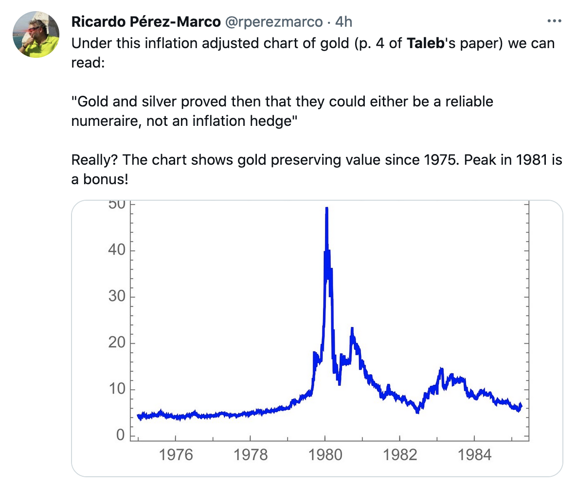
Perez-Marco can’t see the difference between Gold and Silver, nor can he get the difference between raw and inflation adjusted chart. Aside from the fact that he doesn’t get the notion of maximumdrawdown as a measure of riskiness.
Selgin
Cato’s institute George Selgin said a looooot of vague things (with some erroneous financial reasoning ) but has not said anything about the paper.
You have zero probability of making money. But it is a great trade.
One-tailed distributions entangle scale and skewness. When you increase the scale, their asymmetry pushes the mass to the right rather than bulge it in the middle. They also illustrate the difference between probability and expectation as well as the difference between various modes of convergence.
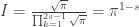
Consider a lognormal with the following parametrization, corresponding to the CDF .
The mean , does not include the parameter thanks to the adjustment in the first parameter. But the standard deviation does, as .
When goes to , the probability of exceeding any positive goes to 0 while the expectation remains invariant. It is because it masses like a Dirac stick at with an infinitesimal mass at infinity which gives it a constant expectation. For the lognormal belongs to the log-location-scale family.
Option traders experience an even worse paradox, see my Dynamic Hedging. As the volatility increases, the delta of the call goes to 1 while the probability of exceeding the strike, any strike, goes to .
More generally, a has for mean, STD, and CDF respectively. We can find a parametrization producing weird behavior in time as .
Thanks: Micah Warren who presented a similar paradox on Twitter.
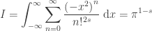
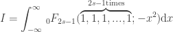
We can start as follows, by transforming it into a generalized hypergeometric function:
, since, from the series expansion of the generalized hypergeometric function, , where is the Pochhammer symbol .
Now the integrand function does not appear to be convergent numerically, except for where it becomes the Gaussian integral, and the case of where it becomes a Bessel function. For and , the integrand takes values of (serious). Beyond that the computer starts to produce smoke. Yet it eventually converges as there is a closed form solution. It is like saying that it works in theory but not in practice!
For, it turns out, under the restriction that , we can use the following result:
Allora, we can substitute , and with , given that ,
.
So either the integrand eventually converges, or I am doing something wrong, or both. Perhaps neither.
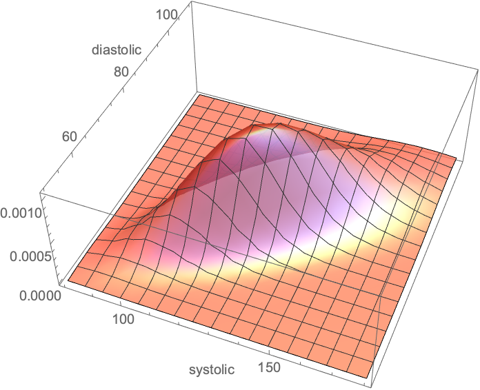
Background: We’ve discussed blood pressure recently with the error of mistaking the average ratio of systolic over diastolic for the ratio of the average of systolic over diastolic. I thought that a natural distribution would be the gamma and cousins, but, using the Framingham data, it turns out that the lognormal works better. For one-tailed distribution, we do not have a lot of choise in handling higher dimensional vectors. There is some literature on the multivariate gamma but it is neither computationally convenient nor a particular good fit.
Well, it turns out that the Lognormal has some powerful properties. I’ve shown in a paper (now a chapter in The Statistical Consequences of Fat Tails) that, under some parametrization (high variance), it can be nearly as “fat-tailed” as the Cauchy. And, under low variance, it can be as tame as the Gaussian. These academic disputes on whether the data is lognormally or power law distributed are totally useless. Here we realize that by using the method of dual distribution, explained below, we can handle matrices rather easily. Simply, if are jointly lognormally distributed with a covariance matrix , then are normally distributed with a matrix . As to the transformation , we will see the operation below.
Let be joint distributed lognormal variables with means and a covariance matrix
allora follow a normal distribution with means and covariance matrix
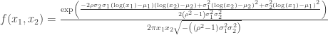
So we can fit one from the other. The pdf for the joint distribution for the lognormal variables becomes:
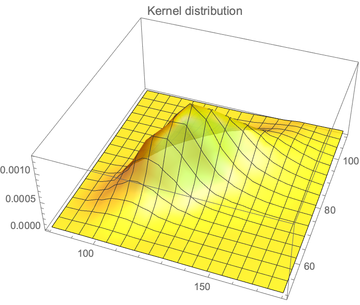
Bivariate Lognormal Distribution
Kernel Distribution
We have the data from the Framingham database for, using for the systolic and for the diastolic, with , which maps to: .


 .
.  ,
, 

 ,
, ,
, ,
, :
:
 , where
  be a vector representing an n sample of independent Bernouilli distributed random variables
  . We are interested in the estimation of the probability p.
 (by reflecting the maximum ignorance point) is
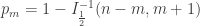 , (1)
, (1) and
and  is the beta regularized function.
  , which clearly does not provide information for small samples.
 , which is not trivial: one is contrained by the fact that matching the mean and variance of the Beta distribution constrains the shape of the prior. Then it becomes convenient that the Beta, being a conjugate prior, updates into the same distribution with new parameters. Allora, with n samples and m realizations:
 (2)
(2) . We will see below how a low variance beta has too much impact on the result.
 be the CDF of the binomial
  . We are interested in
  the maximum entropy probability. First let us figure out the target value q.
 . This is a very standard result: taking the first derivative w.r. to q,
  and since
  is concave to q, we get
  .
. .
. ;
; .
.
 a binomially distributed r.v.
  where n is the number of trials and
  .
. and
and  , we have
  .
. , we can eliminate one parameter. Let us say we start with
  and have no idea of the variance. As we can see in the graph below there are a lot of shapes to the possible distribution: it becomes all in the parametrization.
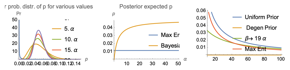


 with the following parametrization,
 ![\mathcal{LN}\left[\mu t-\frac{\sigma ^2 t}{2},\sigma \sqrt{t}\right]](https://s0.wp.com/latex.php?latex=%5Cmathcal%7BLN%7D%5Cleft%5B%5Cmu+t-%5Cfrac%7B%5Csigma+%5E2+t%7D%7B2%7D%2C%5Csigma+%5Csqrt%7Bt%7D%5Cright%5D&bg=ffffff&fg=333333&s=0&c=20201002) corresponding to the CDF
corresponding to the CDF 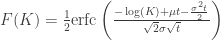 .
. , does not include the parameter
  thanks to the
  adjustment in the first parameter. But the standard deviation does, as
  .
. , the probability of exceeding any positive
  goes to 0 while the expectation remains invariant. It is because it masses like a Dirac stick at
![\mathcal{LN}[a,b]](https://s0.wp.com/latex.php?latex=%5Cmathcal%7BLN%7D%5Ba%2Cb%5D&bg=ffffff&fg=333333&s=0&c=20201002) has for mean, STD, and CDF
has for mean, STD, and CDF  respectively. We can find a parametrization producing weird behavior in time as
  .
. .
. , since, from the series expansion of the generalized hypergeometric function,
  , where
  is the Pochhammer symbol
  .
. where it becomes the Gaussian integral, and the case of
  where it becomes a Bessel function. For
  and
and  , the integrand takes values of
  (serious). Beyond that the computer starts to produce smoke. Yet it eventually converges as there is a closed form solution. It is like saying that it works in theory but not in practice!
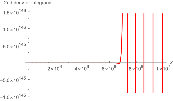
 , we can use the following result:
 , and with
  , given that
  ,
,  .
. are jointly lognormally distributed with a covariance matrix
  , then
  are normally distributed with a matrix
  . As to the transformation
  , we will see the operation below.
 be joint distributed lognormal variables with means
  and a covariance matrix
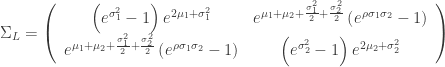
 follow a normal distribution with means
  and covariance matrix
 for the systolic and
  for the diastolic, with
  , which maps to:
  .
.