Probability

Background: We’ve discussed blood pressure recently with the error of mistaking the average ratio of systolic over diastolic for the ratio of the average of systolic over diastolic. I thought that a natural distribution would be the gamma and cousins, but, using the Framingham data, it turns out that the lognormal works better. For one-tailed distribution, we do not have a lot of choise in handling higher dimensional vectors. There is some literature on the multivariate gamma but it is neither computationally convenient nor a particular good fit.

Well, it turns out that the Lognormal has some powerful properties. I’ve shown in a paper (now a chapter in The Statistical Consequences of Fat Tails) that, under some parametrization (high variance), it can be nearly as “fat-tailed” as the Cauchy. And, under low variance, it can be as tame as the Gaussian. These academic disputes on whether the data is lognormally or power law distributed are totally useless. Here we realize that by using the method of dual distribution, explained below, we can handle matrices rather easily. Simply, if $Y_1, Y_2, \ldots Y_n$ are jointly lognormally distributed with a covariance matrix $\Sigma_L$ , then $\log(Y_1), \log(Y_2), \ldots \log(Y_n)$ are normally distributed with a matrix $\Sigma_N$ . As to the transformation $\Sigma_L \to \Sigma_N$ , we will see the operation below.

Let $X_1=x_{1,1},\ldots,x_{1,n}, X_2= x_{2,1},\dots x_{2,n}$ be joint distributed lognormal variables with means $\left(e^{\mu _1+\frac{\sigma _1^2}{2}}, e^{\mu _2+\frac{\sigma _2^2}{2}}\right)$ and a covariance matrix

$\Sigma_L=\left(\begin{array}{cc}\left(e^{\sigma _1^2}-1\right) e^{2 \mu _1+\sigma _1^2}&e^{\mu _1+\mu _2+\frac{\sigma _1^2}{2}+\frac{\sigma _2^2}{2}}\left(e^{\rho \sigma _1 \sigma _2}-1\right)\\ e^{\mu _1+\mu _2+\frac{\sigma _1^2}{2}+\frac{\sigma _2^2}{2}}\left(e^{\rho \sigma _1 \sigma _2}-1\right)&\left(e^{\sigma _2^2}-1\right) e^{2 \mu _2+\sigma _2^2}\end{array}\right)$

allora $\log(x_{1,1}),\ldots, \log(x_{1,n}), \log(x_{2,1}),\dots \log(x_{2,n})$ follow a normal distribution with means $(\mu_1, \mu_2)$ and covariance matrix

$\Sigma_N=\left(\begin{array}{cc}\sigma _1^2&\rho \sigma _1 \sigma _2 \\ \rho \sigma _1 \sigma _2&\sigma _2^2 \\ \end{array}\right)$

So we can fit one from the other. The pdf for the joint distribution for the lognormal variables becomes:

$f(x_1,x_2)= \frac{\exp \left(\frac{-2 \rho \sigma _2 \sigma _1 \left(\log \left(x_1\right)-\mu _1\right) \left(\log \left(x_2\right)-\mu _2\right)+\sigma _1^2 \left(\log \left(x_2\right)-\mu _2\right){}^2+\sigma _2^2 \left(\log \left(x_1\right)-\mu _1\right){}^2}{2 \left(\rho ^2-1\right) \sigma _1^2 \sigma _2^2}\right)}{2 \pi x_1 x_2 \sqrt{-\left(\left(\rho ^2-1\right) \sigma _1^2 \sigma _2^2\right)}}$

We have the data from the Framingham database for, using $X_1$ for the systolic and $X_2$ for the diastolic, with $n=4040, Y_1= \log(X_1), Y_2=\log(X_2): {\mu_1=4.87,\mu_2=4.40, \sigma_1=0.1575, \sigma_2=0.141, \rho= 0.7814}$ , which maps to: ${m_1=132.35, m_2= 82.89, s_1= 22.03, s_2=11.91}$ .

The Lancet article: Maron, Barry J., and Paul D. Thompson. “Longevity in elite athletes: the first 4-min milers.” The Lancet 392, no. 10151 (2018): 913 contains an eggregious probabilistic mistake in handling “expectancy” a severely misunderstood –albeit basic– mathematical operator. It is the same mistake you read in the journalistic “evidence based” literature about ancient people having short lives (discussed in Fooled by Randomness), that they had a life expectancy (LE) of 40 years in the past and that we moderns are so much better thanks to cholesterol lowering pills. Something elementary: unconditional life expectancy at birth includes all people who are born. If only half die at birth, and the rest live 80 years, LE will be ~40 years. Now recompute with the assumption that 75% of children did not make it to their first decade and you will see that life expectancy is a statement of, mostly, child mortality. It is front-loaded. As child mortality has decreased in the last few decades, it is less front-loaded but it is cohort-significant.

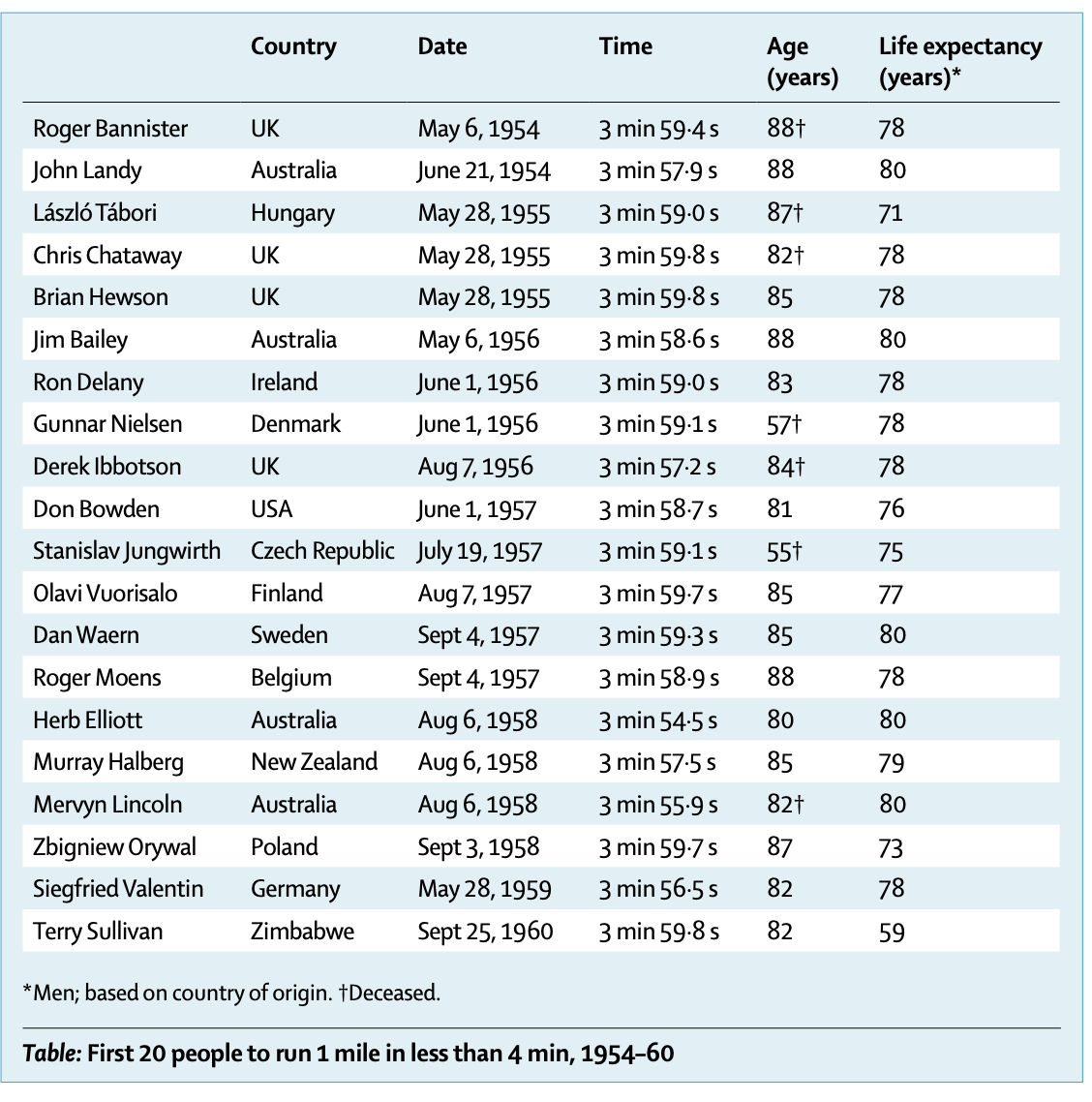
The article (see the Table below) compares the life expectancy of athletes in a healthy cohort of healthy adults to the LE at birth of the country of origin. Their aim was to debunk the theory that while exercise is good, there is a nonlinear dose-response and extreme exercise backfires.

Something even more elementary missed in the Lancet article. If you are a nonsmoker, healthy enough to run a mile (at any speed), do not engage in mafia activities, do not do drugs, do not have metabolic syndrome, do not do amateur aviation, do not ride a motorcycle, do not engage in pro-Trump rioting on Capitol Hill, etc., then unconditional LE has nothing to do with you. Practically nothing.

Just consider that 17% of males today smoke (and perhaps twice as much at the time of the events in the “Date” column of the table). Smoking reduces your life expectancy by about 10 years. Also consider that a quarter or so of Americans over 18 and more than half of those over 50 have metabolic syndrome (depending on how it is defined).

Lindy and NonLindy

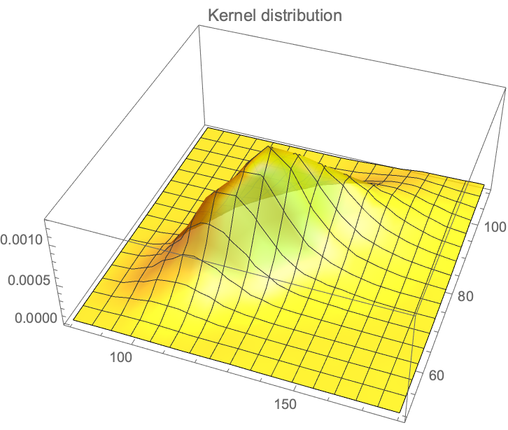
Now some math. What is the behavior of life expectancy over time?

Let $X$ be a random variable that lives in $(0,\infty)$ and $\mathbb{E}$ the expectation operator under “real world” (physical) distribution. By classical results, see the exact exposition in The Statistical Consequences of Fat Tails:

$\lim_{K \to \infty} \frac{1}{K} \mathbb{E}(X|_{X>K})= \lambda$

If $\lambda=1$ , $X$ is said to be in the thin tailed class $\mathcal{D}_1$ and has a characteristic scale . It means life expectancy decreases with age, owing to senescence, or, more rigorously, an increase of the force of mortality/hazard rate over time.

If $\lambda>1$ , $X$ is said to be in the fat tailed regular variation class $\mathcal{D}2$ and has no characteristic scale. This is the Lindy effect where life expectancy increases with age.

If $\lim_{K \to \infty} \mathbb{E}(X|_{X>K})-K= \lambda$ where $\lambda >0$ , then $X$ is in the borderline exponential class.

The next conversation will be about the controversy as to whether human centenarians, after aging is done, enter the third class, just like crocodiles observed in the wild, where LE is a flat number (but short) regardless of age. It may be around 2 years whether one is 100 or 120.

N N Taleb's Probability Notebook

Mathematical flaneuring, almost always probability

Menu

On the Multivariate Lognormal with Application to Blood Pressure

Some (mis)Understanding of life Expectancy, with some good news.

Lindy and NonLindy