You have zero probability of making money. But it is a great trade.
One-tailed distributions entangle scale and skewness. When you increase the scale, their asymmetry pushes the mass to the right rather than bulge it in the middle. They also illustrate the difference between probability and expectation as well as the difference between various modes of convergence.
Consider a lognormal 
![\mathcal{LN}\left[\mu t-\frac{\sigma ^2 t}{2},\sigma \sqrt{t}\right]](https://s0.wp.com/latex.php?latex=%5Cmathcal%7BLN%7D%5Cleft%5B%5Cmu+t-%5Cfrac%7B%5Csigma+%5E2+t%7D%7B2%7D%2C%5Csigma+%5Csqrt%7Bt%7D%5Cright%5D&bg=ffffff&fg=333333&s=0&c=20201002)
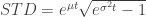
The mean 


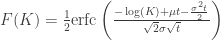
When 


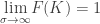
Option traders experience an even worse paradox, see my Dynamic Hedging. As the volatility increases, the delta of the call goes to 1 while the probability of exceeding the strike, any strike, goes to
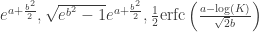
More generally, a ![\mathcal{LN}[a,b]](https://s0.wp.com/latex.php?latex=%5Cmathcal%7BLN%7D%5Ba%2Cb%5D&bg=ffffff&fg=333333&s=0&c=20201002)

Thanks: Micah Warren who presented a similar paradox on Twitter.
