
Financial theory requires correlation to be constant (or, at least, known and nonrandom). Nonrandom means predictable with waning sampling error over the period concerned. Ellipticality is a condition more necessary than thin tails, recall my Twitter fight with that non-probabilist Clifford Asness where I questioned not just his empirical claims and his real-life record, but his own theoretical rigor and the use by that idiot Antti Ilmanen of cartoon models to prove a point about tail hedging. Their entire business reposes on that ghost model of correlation-diversification from modern portfolio theory. The fight was interesting sociologically, but not technically. What is interesting technically is the thingy below.
How do we extract sampling error of a rolling correlation? My coauthor and I could not find it in the literature so we derive the test statistics. The result: it has less than 
The derivations are as follows:
Let 


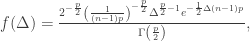
First, we consider the distribution of the Pearson correlation for 
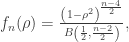
with characteristic function:

where 
We can assert that, for 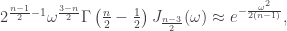
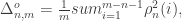
Moments of order 
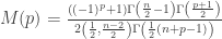
where 


This allows us to treat the distribution of 


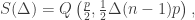
To test how the second moment of the sample coefficient compares to that of a random series, and thanks to the assumption of a mean of
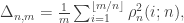
where 
where 

and survival function:

which allows us to obtain p-values below, using 

Such low p-values exclude any controversy as to their effectiveness cite{taleb2016meta}.
We can also compare rolling correlations using a Monte Carlo for the null with practically the same results (given the exceedingly low p-values). We simulate 
Rolling windows have the same second moment, but a mildly more compressed distribution since the observations of 


[…] Talking of put/call ratios and odd correlations- here’s the randomness guv’nor Nassim Taleb: https://fooledbyrandomnessdotcom.wordpress.com/2021/11/24/detecting-bs-in-correlation-windows/ […]
LikeLike