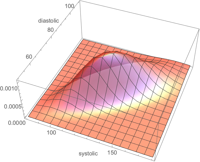
Background: We’ve discussed blood pressure recently with the error of mistaking the average ratio of systolic over diastolic for the ratio of the average of systolic over diastolic. I thought that a natural distribution would be the gamma and cousins, but, using the Framingham data, it turns out that the lognormal works better. For one-tailed distribution, we do not have a lot of choise in handling higher dimensional vectors. There is some literature on the multivariate gamma but it is neither computationally convenient nor a particular good fit.
Well, it turns out that the Lognormal has some powerful properties. I’ve shown in a paper (now a chapter in The Statistical Consequences of Fat Tails) that, under some parametrization (high variance), it can be nearly as “fat-tailed” as the Cauchy. And, under low variance, it can be as tame as the Gaussian. These academic disputes on whether the data is lognormally or power law distributed are totally useless. Here we realize that by using the method of dual distribution, explained below, we can handle matrices rather easily. Simply, if are jointly lognormally distributed with a covariance matrix , then are normally distributed with a matrix . As to the transformation , we will see the operation below.
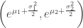
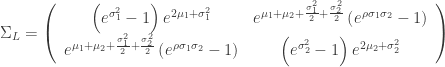
Let be joint distributed lognormal variables with means and a covariance matrix
allora follow a normal distribution with means and covariance matrix
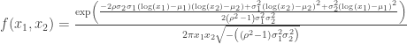
So we can fit one from the other. The pdf for the joint distribution for the lognormal variables becomes:
Bivariate Lognormal Distribution
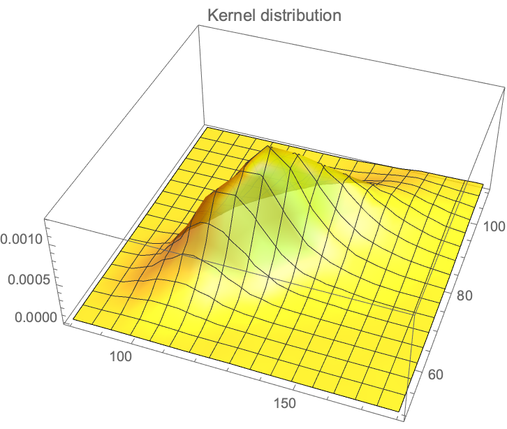
Kernel Distribution
We have the data from the Framingham database for, using for the systolic and for the diastolic, with , which maps to: .
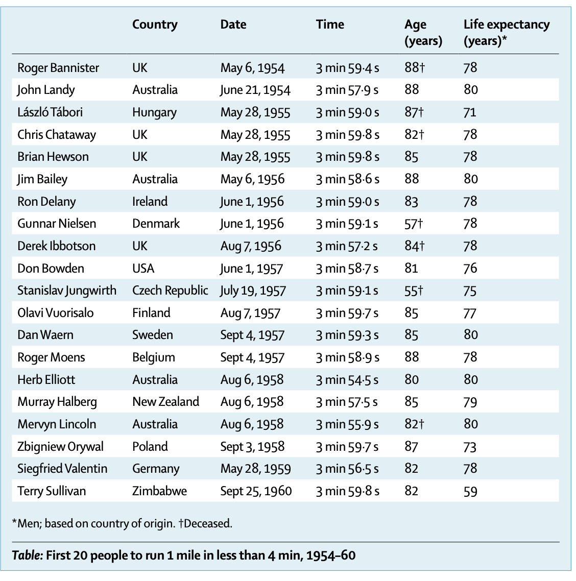
The Lancet article: Maron, Barry J., and Paul D. Thompson. “Longevity in elite athletes: the first 4-min milers.” The Lancet 392, no. 10151 (2018): 913 contains an eggregious probabilistic mistake in handling “expectancy” a severely misunderstood –albeit basic– mathematical operator. It is the same mistake you read in the journalistic “evidence based” literature about ancient people having short lives (discussed in Fooled by Randomness), that they had a life expectancy (LE) of 40 years in the past and that we moderns are so much better thanks to cholesterol lowering pills. Something elementary: unconditional life expectancy at birth includes all people who are born. If only half die at birth, and the rest live 80 years, LE will be ~40 years. Now recompute with the assumption that 75% of children did not make it to their first decade and you will see that life expectancy is a statement of, mostly, child mortality. It is front-loaded. As child mortality has decreased in the last few decades, it is less front-loaded but it is cohort-significant.
The article (see the Table below) compares the life expectancy of athletes in a healthy cohort of healthyadults to the LE at birth of the country of origin. Their aim was to debunk the theory that while exercise is good, there is a nonlinear dose-response and extreme exercise backfires.
Something even more elementary missed in the Lancet article. If you are a nonsmoker, healthy enough to run a mile (at any speed), do not engage in mafia activities, do not do drugs, do not have metabolic syndrome, do not do amateur aviation, do not ride a motorcycle, do not engage in pro-Trump rioting on Capitol Hill, etc., then unconditional LE has nothing to do with you. Practically nothing.
Just consider that 17% of males today smoke (and perhaps twice as much at the time of the events in the “Date” column of the table). Smoking reduces your life expectancy by about 10 years. Also consider that a quarter or so of Americans over 18 and more than half of those over 50 have metabolic syndrome (depending on how it is defined).
Lindy and NonLindy
Now some math. What is the behavior of life expectancy over time?
Let be a random variable that lives in and the expectation operator under “real world” (physical) distribution. By classical results, see the exact exposition in The Statistical Consequences of Fat Tails:
If , is said to be in the thin tailed class and has a characteristic scale . It means life expectancy decreases with age, owing to senescence, or, more rigorously, an increase of the force of mortality/hazard rate over time.
If , is said to be in the fat tailed regular variation class and has no characteristic scale. This is the Lindy effect where life expectancy increases with age.
If where , then is in the borderline exponential class.
The next conversation will be about the controversy as to whether human centenarians, after aging is done, enter the third class, just like crocodiles observed in the wild, where LE is a flat number (but short) regardless of age. It may be around 2 years whether one is 100 or 120.
In Yalta, K., Ozturk, S., & Yetkin, E. (2016). “Golden Ratio and the heart: A review of divine aesthetics”, International Journal of Cardiology, 214, 107-112, the authors compute the ambulatory ratio of Systolic to Diastolic by averaging each and taking the ratio. “Mean values of diastolic and systolic pressure levels during 24-h, day-time and night-time recordings were assessed to calculate the ratios of SBP/DBP and DBP/PP in these particular periods”.
The error is to compute the mean SBP and mean DBP then get the ratio, rather than compute every SBP/DBP data point. Simply,
Easy to see with just n=2: .
The rest is mathematical considerations until I get real data to find the implication of this error that seems to have seeped through the literature (we know there is an eggregious mathematical error; how severe the consequences need to be assessed from data.). For the intuition of the problem consider that when people tell you that healthy people have on average BP of 120/80, that those whose systolic is 120 must have a diastolic 80, and vice-versa, which can only be true if the ratio is deterministic .
Clearly, from Jensen’s inequality, where and are random variables, whether independent or dependent, correlated or uncorrelated, we have:
with few exceptions, s.a. a perfectly correlated (positively or negatively) and in which case the equality is forced by the fact that the ratio becomes a degenerate random variable.
Inequality: At the core lies the fundamental ratio inequality (by Jensen’s) that:
,
or . The proof is easy: is a convex function of y and has a positive second derivative.
Allora when and are independent, we have the ratio distribution
Furthermore, where the two variables have support on , say a Gaussian distribution , the mean of the ratio is infinite. How? Simply , for ,
From where we can work out the counterintuitive result that if and and respectively,
,
with infinite moments. As a nice exercise we can get the exact PDF under some correlation structure in a bivariate normal:
,
with a mean that exists only if (that is will be 0 in the exactly symmetric case).
Luckily, SBP () and DBP () live in which should yield a finite mean and allow us to use Mellin’s transform which is a good warm up after the holidays (while witing for the magisterial Algebra of Random Variables to arrive by mail).
Note: For a lognormal distribution parametrized with , under independence:
Owing to the fact that the ratio follows another lognormal with for parameters .
Gamma: I’ve calibrated from various papers that it must be a gamma distribution with standard deviations of 14-24 and 10-14 respectively. There are papers on bivariate (multivariate) gamma distributions in the statistics literature (though nothing in the DSBR, the “Data Science Bullshitters Recipes”), but on this distribution later. We can work out that if (gamma) and , assuming independence (for now), we have the ratio
with mean while .
Assuming Gamma Distribution
Pierre Zalloua has promised me 10,000 BP observations so we can compute the ratios under a correlation structure.


 be a random variable that lives in
  and
and  the expectation operator under “real world” (physical) distribution. By classical results, see the exact exposition in The Statistical Consequences of Fat Tails:
 ,
,  and has a characteristic scale . It means life expectancy decreases with age, owing to senescence, or, more rigorously, an increase of the force of mortality/hazard rate over time.
 ,
,  and has no characteristic scale. This is the Lindy effect where life expectancy increases with age.
 where
where  , then
 .
. are random variables, whether independent or dependent, correlated or uncorrelated, we have:
 ,
, . The proof is easy:
  is a convex function of y and has a positive second derivative.
 , say a Gaussian distribution
  , the mean of the ratio is infinite. How? Simply , for
  ,
,


 and
and  respectively,
  ,
,  in a bivariate normal:
  ,
, that exists only if
  (that is will be 0 in the exactly symmetric case).
 which should yield a finite mean and allow us to use Mellin’s transform which is a good warm up after the holidays (while witing for the magisterial Algebra of Random Variables to arrive by mail).
  , under independence:
![\left[\mu _1-\mu _2,\sqrt{\sigma _1^2+\sigma _2^2}\right]](https://s0.wp.com/latex.php?latex=%5Cleft%5B%5Cmu+_1-%5Cmu+_2%2C%5Csqrt%7B%5Csigma+_1%5E2%2B%5Csigma+_2%5E2%7D%5Cright%5D&bg=ffffff&fg=333333&s=0&c=20201002) .
. (gamma) and
  , assuming independence (for now), we have the ratio

 while
while  .
.
