The Lancet article: Maron, Barry J., and Paul D. Thompson. “Longevity in elite athletes: the first 4-min milers.” The Lancet 392, no. 10151 (2018): 913 contains an eggregious probabilistic mistake in handling “expectancy” a severely misunderstood –albeit basic– mathematical operator. It is the same mistake you read in the journalistic “evidence based” literature about ancient people having short lives (discussed in Fooled by Randomness), that they had a life expectancy (LE) of 40 years in the past and that we moderns are so much better thanks to cholesterol lowering pills. Something elementary: unconditional life expectancy at birth includes all people who are born. If only half die at birth, and the rest live 80 years, LE will be ~40 years. Now recompute with the assumption that 75% of children did not make it to their first decade and you will see that life expectancy is a statement of, mostly, child mortality. It is front-loaded. As child mortality has decreased in the last few decades, it is less front-loaded but it is cohort-significant.
The article (see the Table below) compares the life expectancy of athletes in a healthy cohort of healthyadults to the LE at birth of the country of origin. Their aim was to debunk the theory that while exercise is good, there is a nonlinear dose-response and extreme exercise backfires.
Something even more elementary missed in the Lancet article. If you are a nonsmoker, healthy enough to run a mile (at any speed), do not engage in mafia activities, do not do drugs, do not have metabolic syndrome, do not do amateur aviation, do not ride a motorcycle, do not engage in pro-Trump rioting on Capitol Hill, etc., then unconditional LE has nothing to do with you. Practically nothing.
Just consider that 17% of males today smoke (and perhaps twice as much at the time of the events in the “Date” column of the table). Smoking reduces your life expectancy by about 10 years. Also consider that a quarter or so of Americans over 18 and more than half of those over 50 have metabolic syndrome (depending on how it is defined).
Lindy and NonLindy
Now some math. What is the behavior of life expectancy over time?
Let be a random variable that lives in and the expectation operator under “real world” (physical) distribution. By classical results, see the exact exposition in The Statistical Consequences of Fat Tails:
If , is said to be in the thin tailed class and has a characteristic scale . It means life expectancy decreases with age, owing to senescence, or, more rigorously, an increase of the force of mortality/hazard rate over time.
If , is said to be in the fat tailed regular variation class and has no characteristic scale. This is the Lindy effect where life expectancy increases with age.
If where , then is in the borderline exponential class.
The next conversation will be about the controversy as to whether human centenarians, after aging is done, enter the third class, just like crocodiles observed in the wild, where LE is a flat number (but short) regardless of age. It may be around 2 years whether one is 100 or 120.
In Yalta, K., Ozturk, S., & Yetkin, E. (2016). “Golden Ratio and the heart: A review of divine aesthetics”, International Journal of Cardiology, 214, 107-112, the authors compute the ambulatory ratio of Systolic to Diastolic by averaging each and taking the ratio. “Mean values of diastolic and systolic pressure levels during 24-h, day-time and night-time recordings were assessed to calculate the ratios of SBP/DBP and DBP/PP in these particular periods”.
The error is to compute the mean SBP and mean DBP then get the ratio, rather than compute every SBP/DBP data point. Simply,
Easy to see with just n=2: .
The rest is mathematical considerations until I get real data to find the implication of this error that seems to have seeped through the literature (we know there is an eggregious mathematical error; how severe the consequences need to be assessed from data.). For the intuition of the problem consider that when people tell you that healthy people have on average BP of 120/80, that those whose systolic is 120 must have a diastolic 80, and vice-versa, which can only be true if the ratio is deterministic .
Clearly, from Jensen’s inequality, where and are random variables, whether independent or dependent, correlated or uncorrelated, we have:
with few exceptions, s.a. a perfectly correlated (positively or negatively) and in which case the equality is forced by the fact that the ratio becomes a degenerate random variable.
Inequality: At the core lies the fundamental ratio inequality (by Jensen’s) that:
,
or . The proof is easy: is a convex function of y and has a positive second derivative.
Allora when and are independent, we have the ratio distribution
Furthermore, where the two variables have support on , say a Gaussian distribution , the mean of the ratio is infinite. How? Simply , for ,
From where we can work out the counterintuitive result that if and and respectively,
,
with infinite moments. As a nice exercise we can get the exact PDF under some correlation structure in a bivariate normal:
,
with a mean that exists only if (that is will be 0 in the exactly symmetric case).
Luckily, SBP () and DBP () live in which should yield a finite mean and allow us to use Mellin’s transform which is a good warm up after the holidays (while witing for the magisterial Algebra of Random Variables to arrive by mail).
Note: For a lognormal distribution parametrized with , under independence:
Owing to the fact that the ratio follows another lognormal with for parameters .
Gamma: I’ve calibrated from various papers that it must be a gamma distribution with standard deviations of 14-24 and 10-14 respectively. There are papers on bivariate (multivariate) gamma distributions in the statistics literature (though nothing in the DSBR, the “Data Science Bullshitters Recipes”), but on this distribution later. We can work out that if (gamma) and , assuming independence (for now), we have the ratio
with mean while .
Assuming Gamma Distribution
Pierre Zalloua has promised me 10,000 BP observations so we can compute the ratios under a correlation structure.
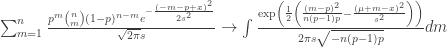
The Danish Mask Study presents the interesting probability problem: the odds of getting 5 infections for a group of 2470, vs 0 for one of 2398. It warrants its own test statistic which allows us to look at all conditional probabilities. Given that we are dealing with tail probabilities, normal approximations are totally out of order. Further we have no idea from the outset on whether the sample size is sufficient to draw conclusions from such a discrepancy (it is). There appears to be no exact distribution in the literatrue for when both and are binomially distributed with different probabilities. Let’s derive it.
Let , , both independent.
We have the constrained probability mass for the joint :
,
with .
For each “state” in the lattice, we need to sum up he ways we can get a given total times the probability, which depends on the number of partitions. For instance:
Every study needs its own statistical tools, adapted to the specific problem, which is why it is a good practice to require that statisticians come from mathematical probability rather than some software-cookbook school. When one uses canned software statistics adapted to regular medicine (say, cardiology), one is bound to make severe mistakes when it comes to epidemiological problems in the tails or ones where there is a measurement error. The authors of the study discussed below (The Danish Mask Study) both missed the effect of false positive noise on sample size and a central statistical signal from a divergence in PCR results. A correct computation of the odds ratio shows a massive risk reduction coming from masks.
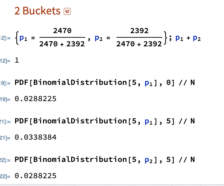
The article by Bundgaard et al., [“Effectiveness of Adding a Mask Recommendation to Other Public Health Measures to Prevent SARS-CoV-2 Infection in Danish Mask Wearers”, Annals of Internal Medicine (henceforth the “Danish Mask Study”)] relies on the standard methods of randomized control trials to establish the difference between the rate of infections of people wearing masks outside the house v.s. those who don’t (the control group), everything else maintained constant. The authors claimed that they calibrated their sample size to compute a p-value (alas) off a base rate of 2% infection in the general population. The result is a small difference in the rate of infection in favor of masks (2.1% vs 1.8%, or 42/2392 vs. 53/2470), deemed by the authors as not sufficient to warrant a conclusion about the effectiveness of masks.
We would like to alert the scientific community to the following :
The Mask Group has 0/2392 PCR infections vs 5/2470 for the Control Group. Note that this is the only robust result and the authors did not test to see how nonrandom that can be. They missed on the strongest statistical signal. (One may also see 5 infections vs. 15 if, in addition, one accounts for clinically detected infections.)
Results
The rest, 42/2392 vs. 53/2470, are from antibody tests with a high error rate which need to be incorporated via propagation of uncertainty-style methods on the statistical significance of the results. Intuitively a false positive rate with an expected “true value” is a random variable Binomial Distribution with STD , etc.
False positives must be deducted in the computation of the odds ratio.
The central problem is that both p and the incidence of infection are in the tails!
Immediate result: the study is highly underpowered –except ironically for the PCR and PCR+clinical results that are overwhelming in evidence.
Further:
As most infections happen at home, the study does not inform on masks in general –it uses wrong denominators for the computation of odds ratios (mixes conditional and unconditional risk). Worse, the study is not even applicable to derive information on masks vs. no masks outside the house since during most of the study (April 3 to May 20, 2020), “cafés and restaurants were closed “, conditions too specific and during which the infection rates are severely reduced –tells us nothing about changes in indoor activity. (The study ended June 2, 2020). A study is supposed to isolate a source of risk; such source must be general to periods outside the study (unlike cardiology with unconditional effects).
The study does not take into account the fact that masks might protect others. Clearly this is not cardiology but an interactive system.
Statistical signals compound. One needs to input the entire shebang, not simple individual tests to assess the joint probability of an effect.
Now, some quick technical derivations.
Distribution of the sample under type 2 error
Simple method: Let be random variables in ; we have
with the constraint that .
So follow a multinomial distribution with probabilities .
If we consider , the observable incidence in each group, the variable follows a binomial distribution , with a large share of the variance coming from .
This poses an immediate problem: we are concerned with not . The odds ratio in each sample used by the researchrs is (where M is for the mask condition and N the no mask one); it is diluted by , which can be considerable.
A back of the envelope analysis shows that, in the presence of a false positive rate of just 1%, we have a large gain for masks. It would not be 42/2392 vs. 53/2470 but rather, by adding the known true positives and reducing by the false negatives (approximately):
vs ,
which is at least an overall drop in 47% of incidence for masks, not counting home infections, which, if they were just 1% (half the total claimed by the resarchers), would increase the benefits for masks in a yuuuuuuuge way (up to 100%).
(These numbers are preliminary and need refining).
More advanced method: Let the initial incidence rate (a Gaussian) for a given sample n. Let us incorporate the false negative as all values across. Let be the total sample size, the (net) probability of a false positive. We now have the corrected distribution of the revealed infection count (using a Binomial distribution of the net false positive rate).
Under normal approximation to the binomial:
Allora
which appears to be Gaussian. For we have:
, hence the kurtosis is that of a Gaussian.
As you see the variance goes through the roof. More details would show that the study needs at least 4 times the sample size for the same approach. I have not added false negatives, but these too would increase the variance.
Considerations on the 0/5 PCR results
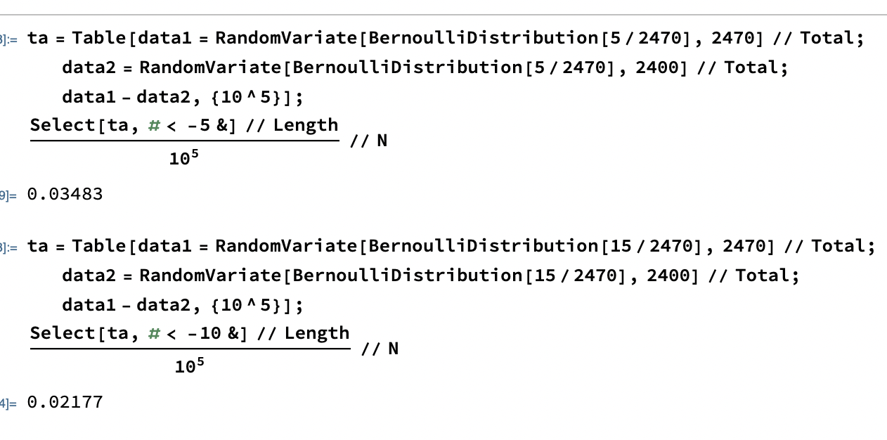
Now consider the more obvious error. What are the odds of getting 0 PCRs vs 5 from random?
The probability of having 0 realizations in 2392 if the mean is is 0.0078518, that is 1 in 127. We can reexpress it in p values, which would be well <.05, that is far in excess of the ps in the range .21-.33 that the paper shows. How these researchers missed the point is beyond me.
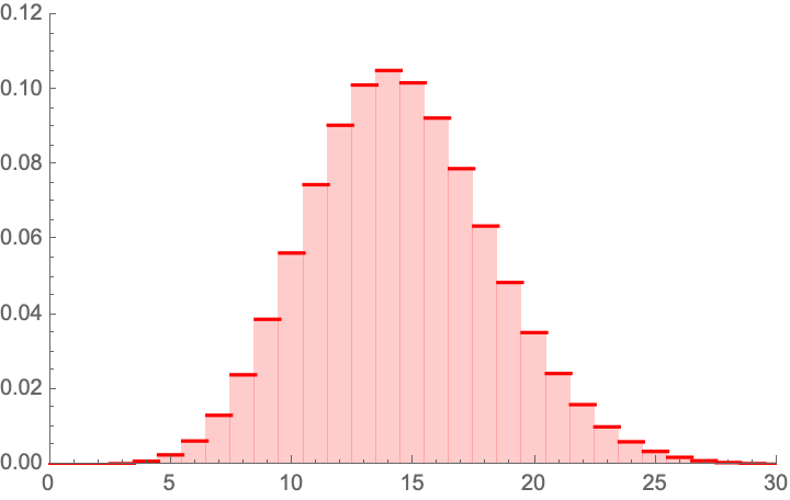
PMF of a binomial distribution(2392 , ) .Another approach Pegadogical presentation of a draw of 5 with the {0,5} combinationMonte Carlo Analysis, again another way.More textbook-style Fisher approach, similar to our heuristic
Considerations on the 5/15 PCR+Clinial detection results
Now consider the 5 vs. 15 PCR + (adjusting the rest)
PMF of a binomial distribution(2392 , ) .
Clinically detected Covid.
The probability of having 5 or less realizations in 2392 if the mean is is 0.00379352, that is 1 in 263. We can reexpress it in p values, which would be well <.1 [CORRECTED based on comments].
(To be continued. I wonder why the journal published a paper with already weak p values, without asking for a repeat with a larger sample which can cure the deficit.)
An interesting discovery, thanks to a problem presented by K. Srinivasa Raghava:
A standard result for real, where is the floor function:
.
Now it so happens that:
which is of course intuitive owing to Riemann surfaces produced by the complex logarithm. I could not find the result but I am nearly certain it must be somewhere.
Now to get an idea, let us examine the compensating function
And of course, the complex logarithm (here is the standard function, just to illustrate):


 .
. are random variables, whether independent or dependent, correlated or uncorrelated, we have:
 ,
, . The proof is easy:
  is a convex function of y and has a positive second derivative.
 , say a Gaussian distribution
  , the mean of the ratio is infinite. How? Simply , for
  ,
,


 and
and  respectively,
  ,
,  in a bivariate normal:
  ,
, that exists only if
  (that is will be 0 in the exactly symmetric case).
 which should yield a finite mean and allow us to use Mellin’s transform which is a good warm up after the holidays (while witing for the magisterial Algebra of Random Variables to arrive by mail).
  , under independence:
![\left[\mu _1-\mu _2,\sqrt{\sigma _1^2+\sigma _2^2}\right]](https://s0.wp.com/latex.php?latex=%5Cleft%5B%5Cmu+_1-%5Cmu+_2%2C%5Csqrt%7B%5Csigma+_1%5E2%2B%5Csigma+_2%5E2%7D%5Cright%5D&bg=ffffff&fg=333333&s=0&c=20201002) .
. (gamma) and
  , assuming independence (for now), we have the ratio

 while
while  .
.
 when both
  and
and  are binomially distributed with different probabilities. Let’s derive it.
 ,
,  , both independent.
 :
: ,
, .
. :
:
 ,
, .
. :
: ,
, (unless I got mixed up with the symbols).


 is a random variable
  Binomial Distribution with STD
  , etc.
  be random variables in
  ; we have
 .
. follow a multinomial distribution with probabilities
  .
. , the observable incidence in each group, the variable follows a binomial distribution
  , with a large share of the variance coming from
  .
. not
not  . The odds ratio in each sample used by the researchrs is
  (where M is for the mask condition and N the no mask one); it is diluted by
  vs
vs 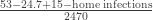 ,
,  (a Gaussian) for a given sample n. Let us incorporate the false negative as all values across. Let
  be the total sample size,
  the corrected distribution of the revealed infection count (using a Binomial distribution of the net false positive rate).


 , hence the kurtosis is that of a Gaussian.
 is 0.0078518, that is 1 in 127. We can reexpress it in p values, which would be well <.05, that is far in excess of the ps in the range .21-.33 that the paper shows. How these researchers missed the point is beyond me.


 ) .
) . real, where
  is the floor function:
 .
.


